kalepy API
Kernel Density Estimation
The primary API is two functions in the top level package: kalepy.density and kalepy.resample. Additionally, kalepy.pdf is included which is a shorthand for kalepy.density(…, probability=True) — i.e. a normalized density distribution.
Each of these functions constructs a KDE (kalepy.kde.KDE) instance, calls the corresponding member function, and returns the results. If multiple operations will be done on the same data set, it will be more efficient to construct the KDE instance manually and call the methods on that. i.e.
kde = kalepy.KDE(data)            # construct `KDE` instance
points, density = kde.density()   # use `KDE` for density-estimation
new_samples = kde.resample()      # use same `KDE` for resampling
Basic Usage
import numpy as np
import matplotlib.pyplot as plt
import matplotlib as mpl

import kalepy as kale

from kalepy.plot import nbshow
Generate some random data, and its corresponding distribution function
NUM = int(1e4)
np.random.seed(12345)
# Combine data from two different PDFs
_d1 = np.random.normal(4.0, 1.0, NUM)
_d2 = np.random.lognormal(0, 0.5, size=NUM)
data = np.concatenate([_d1, _d2])

# Calculate the "true" distribution
xx = np.linspace(0.0, 7.0, 100)[1:]
yy = 0.5*np.exp(-(xx - 4.0)**2/2) / np.sqrt(2*np.pi)
yy += 0.5 * np.exp(-np.log(xx)**2/(2*0.5**2)) / (0.5*xx*np.sqrt(2*np.pi))
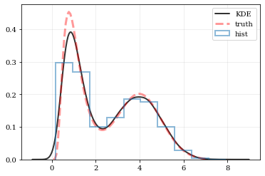
Plotting Smooth Distributions
# Reconstruct the probability-density based on the given data points.
points, density = kale.density(data, probability=True)

# Plot the PDF
plt.plot(points, density, 'k-', lw=2.0, alpha=0.8, label='KDE')

# Plot the "true" PDF
plt.plot(xx, yy, 'r--', alpha=0.4, lw=3.0, label='truth')

# Plot the standard, histogram density estimate
plt.hist(data, density=True, histtype='step', lw=2.0, alpha=0.5, label='hist')

plt.legend()
nbshow()
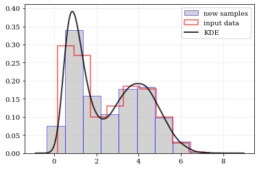
resampling: constructing statistically similar values
Draw a new sample of data-points from the KDE PDF
# Draw new samples from the KDE reconstructed PDF
samples = kale.resample(data)

# Plot new samples
plt.hist(samples, density=True, label='new samples', alpha=0.5, color='0.65', edgecolor='b')
# Plot the old samples
plt.hist(data, density=True, histtype='step', lw=2.0, alpha=0.5, color='r', label='input data')

# Plot the KDE reconstructed PDF
plt.plot(points, density, 'k-', lw=2.0, alpha=0.8, label='KDE')

plt.legend()
nbshow()
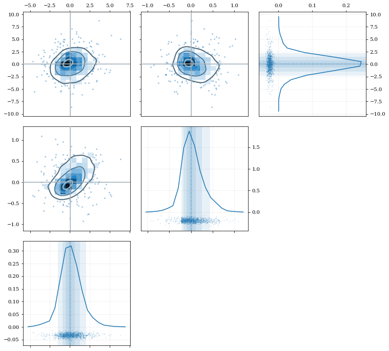
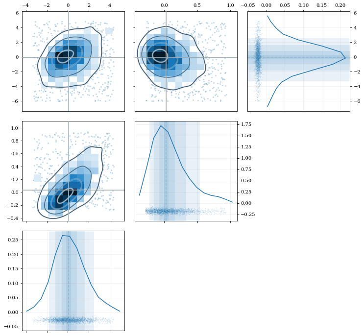
Multivariate Distributions
# Load some random-ish three-dimensional data
data = kale.utils._random_data_3d_02()

# Construct a KDE
kde = kale.KDE(data)

# Plot the data and distributions using the builtin `kalepy.corner` plot
kale.corner(kde)

nbshow()
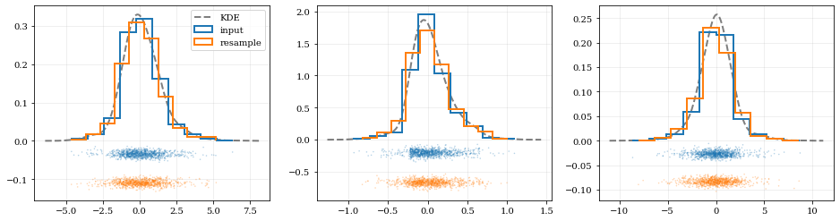
# Resample the data (default output is the same size as the input data)
samples = kde.resample()


# ---- Plot the input data compared to the resampled data ----

fig, axes = plt.subplots(figsize=[16, 4], ncols=kde.ndim)

for ii, ax in enumerate(axes):
    # Calculate and plot PDF for `ii`th parameter (i.e. data dimension `ii`)
    xx, yy = kde.density(params=ii, probability=True)
    ax.plot(xx, yy, 'k--', label='KDE', lw=2.0, alpha=0.5)
    # Draw histograms of original and newly resampled datasets
    *_, h1 = ax.hist(data[ii], histtype='step', density=True, lw=2.0, label='input')
    *_, h2 = ax.hist(samples[ii], histtype='step', density=True, lw=2.0, label='resample')
    # Add 'kalepy.carpet' plots showing the data points themselves
    kale.carpet(data[ii], ax=ax, color=h1[0].get_facecolor())
    kale.carpet(samples[ii], ax=ax, color=h2[0].get_facecolor(), shift=ax.get_ylim()[0])

axes[0].legend()
nbshow()
Fancy Usage
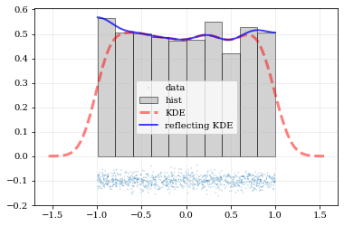
Reflecting Boundaries
What if the distributions you’re trying to capture have edges in them, like in a uniform distribution between two bounds? Here, the KDE chooses ‘reflection’ locations based on the extrema of the given data.
# Uniform data (edges at -1 and +1)
NDATA = 1e3
np.random.seed(54321)
data = np.random.uniform(-1.0, 1.0, int(NDATA))

# Create a 'carpet' plot of the data
kale.carpet(data, label='data')
# Histogram the data
plt.hist(data, density=True, alpha=0.5, label='hist', color='0.65', edgecolor='k')

# ---- Standard KDE will undershoot just-inside the edges and overshoot outside edges
points, pdf_basic = kale.density(data, probability=True)
plt.plot(points, pdf_basic, 'r--', lw=3.0, alpha=0.5, label='KDE')

# ---- Reflecting KDE keeps probability within the given bounds
# setting `reflect=True` lets the KDE guess the edge locations based on the data extrema
points, pdf_reflect = kale.density(data, reflect=True, probability=True)
plt.plot(points, pdf_reflect, 'b-', lw=2.0, alpha=0.75, label='reflecting KDE')

plt.legend()
nbshow()
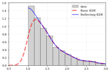
Explicit reflection locations can also be provided (in any number of dimensions).
# Construct random data, add an artificial 'edge'
np.random.seed(5142)
edge = 1.0
data = np.random.lognormal(sigma=0.5, size=int(3e3))
data = data[data >= edge]

# Histogram the data, use fixed bin-positions
edges = np.linspace(edge, 4, 20)
plt.hist(data, bins=edges, density=True, alpha=0.5, label='data', color='0.65', edgecolor='k')

# Standard KDE with over & under estimates
points, pdf_basic = kale.density(data, probability=True)
plt.plot(points, pdf_basic, 'r--', lw=4.0, alpha=0.5, label='Basic KDE')

# Reflecting KDE setting the lower-boundary to the known value
#    There is no upper-boundary when `None` is given.
points, pdf_basic = kale.density(data, reflect=[edge, None], probability=True)
plt.plot(points, pdf_basic, 'b-', lw=3.0, alpha=0.5, label='Reflecting KDE')

plt.gca().set_xlim(edge - 0.5, 3)
plt.legend()
nbshow()
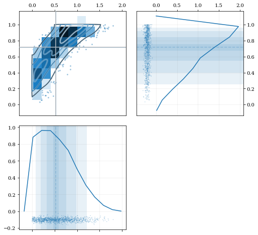
Multivariate Reflection
# Load a predefined dataset that has boundaries at:
#   x: 0.0 on the low-end
#   y: 1.0 on the high-end
data = kale.utils._random_data_2d_03()

# Construct a KDE with the given reflection boundaries given explicitly
kde = kale.KDE(data, reflect=[[0, None], [None, 1]])

# Plot using default settings
kale.corner(kde)

nbshow()
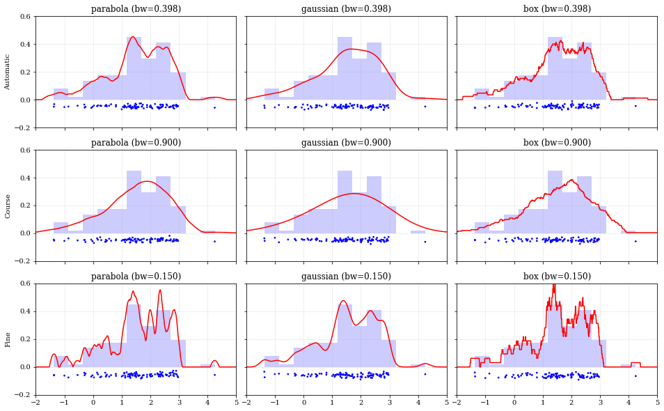
Specifying Bandwidths and Kernel Functions
# Load predefined 'random' data
data = kale.utils._random_data_1d_02(num=100)
# Choose a uniform x-spacing for drawing PDFs
xx = np.linspace(-2, 8, 1000)

# ------ Choose the kernel-functions and bandwidths to test -------  #
kernels = ['parabola', 'gaussian', 'box']                            #
bandwidths = [None, 0.9, 0.15]     # `None` means let kalepy choose  #
# -----------------------------------------------------------------  #

ylabels = ['Automatic', 'Course', 'Fine']
fig, axes = plt.subplots(figsize=[16, 10], ncols=len(kernels), nrows=len(bandwidths), sharex=True, sharey=True)
plt.subplots_adjust(hspace=0.2, wspace=0.05)
for (ii, jj), ax in np.ndenumerate(axes):

    # ---- Construct KDE using particular kernel-function and bandwidth ---- #
    kern = kernels[jj]                                                       #
    bw = bandwidths[ii]                                                      #
    kde = kale.KDE(data, kernel=kern, bandwidth=bw)                          #
    # ---------------------------------------------------------------------- #

    # If bandwidth was set to `None`, then the KDE will choose the 'optimal' value
    if bw is None:
        bw = kde.bandwidth[0, 0]

    ax.set_title('{} (bw={:.3f})'.format(kern, bw))
    if jj == 0:
        ax.set_ylabel(ylabels[ii])

    # plot the KDE
    ax.plot(*kde.pdf(points=xx), color='r')
    # plot histogram of the data (same for all panels)
    ax.hist(data, bins='auto', color='b', alpha=0.2, density=True)
    # plot  carpet   of the data (same for all panels)
    kale.carpet(data, ax=ax, color='b')

ax.set(xlim=[-2, 5], ylim=[-0.2, 0.6])
nbshow()
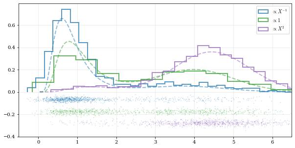
Using different data weights
# Load some random data (and the 'true' PDF, for comparison)
data, truth = kale.utils._random_data_1d_01()

# ---- Resample the same data, using different weightings ---- #
resamp_uni = kale.resample(data, size=1000)                       #
resamp_sqr  = kale.resample(data, weights=data**2, size=1000)      #
resamp_inv = kale.resample(data, weights=data**-1, size=1000)     #
# ------------------------------------------------------------ #


# ---- Plot different distributions ----

# Setup plotting parameters
kw = dict(density=True, histtype='step', lw=2.0, alpha=0.75, bins='auto')

xx, yy = truth
samples = [resamp_inv, resamp_uni, resamp_sqr]
yvals = [yy/xx, yy, yy*xx**2/10]
labels = [r'$\propto X^{-1}$', r'$\propto 1$', r'$\propto X^2$']

plt.figure(figsize=[10, 5])

for ii, (res, yy, lab) in enumerate(zip(samples, yvals, labels)):
    hh, = plt.plot(xx, yy, ls='--', alpha=0.5, lw=2.0)
    col = hh.get_color()
    kale.carpet(res, color=col, shift=-0.1*ii)
    plt.hist(res, color=col, label=lab, **kw)

plt.gca().set(xlim=[-0.5, 6.5])
# Add legend
plt.legend()
# display the figure if this is a notebook
nbshow()
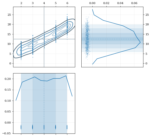
Resampling while ‘keeping’ certain parameters/dimensions
# Construct covariant 2D dataset where the 0th parameter takes on discrete values
xx = np.random.randint(2, 7, 1000)
yy = np.random.normal(4, 2, xx.size) + xx**(3/2)
data = [xx, yy]

# 2D plotting settings: disable the 2D histogram & disable masking of dense scatter-points
dist2d = dict(hist=False, mask_dense=False)

# Draw a corner plot
kale.corner(data, dist2d=dist2d)

nbshow()
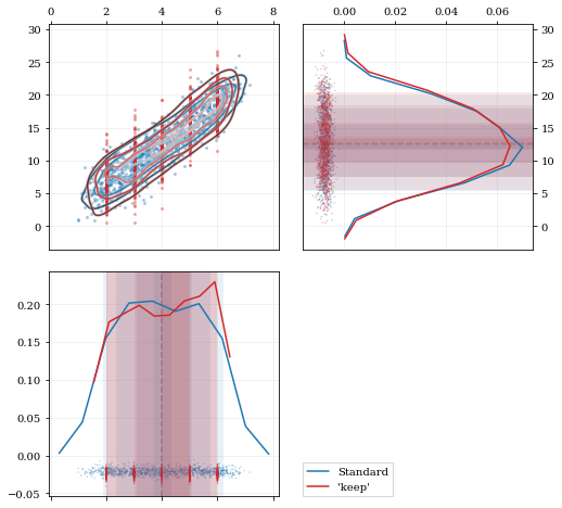
A standard KDE resampling will smooth out the discrete variables,
creating a smooth(er) distribution. Using the keep parameter, we can
choose to resample from the actual data values of that parameter instead
of resampling with ‘smoothing’ based on the KDE.
kde = kale.KDE(data)

# ---- Resample the data both normally, and 'keep'ing the 0th parameter values ---- #
resamp_stnd = kde.resample()                                                        #
resamp_keep = kde.resample(keep=0)                                                  #
# --------------------------------------------------------------------------------- #

corner = kale.Corner(2)
dist2d['median'] = False    # disable median 'cross-hairs'
h1 = corner.plot(resamp_stnd, dist2d=dist2d)
h2 = corner.plot(resamp_keep, dist2d=dist2d)

corner.legend([h1, h2], ['Standard', "'keep'"])
nbshow()
Plotting Distributions
For more extended documentation, see the kalepy.plot submodule documentation.
import kalepy as kale
import numpy as np
import matplotlib.pyplot as plt
kalepy.corner() and the kalepy.Corner class
For the full documentation, see:
Plot some three-dimensional data called data3 with shape (3, N) with
N data points.
kale.corner(data3);
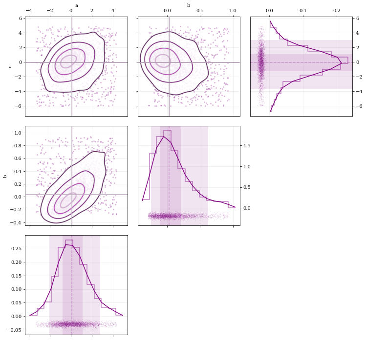
Extensive modifications are possible with passed arguments, for example:
# 1D plot settings: turn on histograms, and modify the confidence-interval quantiles
dist1d = dict(hist=True, quantiles=[0.5, 0.9])
# 2D plot settings: turn off the histograms, and turn on scatter
dist2d = dict(hist=False, scatter=True)

kale.corner(data3, labels=['a', 'b', 'c'], color='purple',
            dist1d=dist1d, dist2d=dist2d);
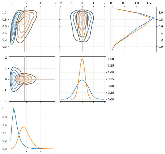
The kalepy.corner method is a wrapper that builds a
kalepy.Corner instance, and then plots the given data. For
additional flexibility, the kalepy.Corner class can be used
directly. This is particularly useful for plotting multiple
distributions, or using preconfigured plotting styles.
# Construct a `Corner` instance for 3 dimensional data, modify the figure size
corner = kale.Corner(3, figsize=[9, 9])

# Plot two different datasets using the `clean` plotting style
corner.clean(data3a)
corner.clean(data3b);
kalepy.dist1d and kalepy.dist2d
The Corner class ultimately calls the functions dist1d and
dist2d to do the actual plotting of each figure panel. These
functions can also be used directly.
For the full documentation, see:
# Plot a 1D dataset, shape: (N,) for `N` data points
kale.dist1d(data1);
# Plot a 2D dataset, shape: (2, N) for `N` data points
kale.dist2d(data2, hist=False);

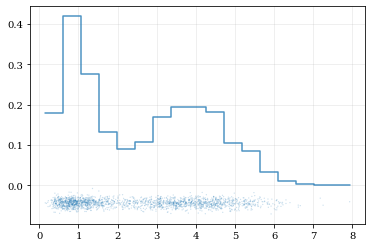
These functions can also be called on a kalepy.KDE instance, which
is particularly useful for utilizing the advanced KDE functionality like
reflection.
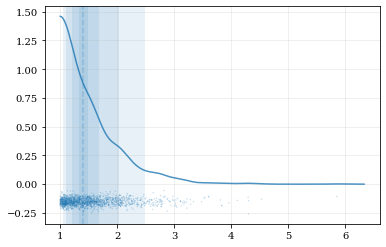
# Construct a random dataset, and truncate it on the left at 1.0
import numpy as np
data = np.random.lognormal(sigma=0.5, size=int(3e3))
data = data[data >= 1.0]

# Construct a KDE, and include reflection (only on the lower/left side)
kde_reflect = kale.KDE(data, reflect=[1.0, None])
# plot, and include confidence intervals
hr = kale.dist1d(kde_reflect, confidence=True);
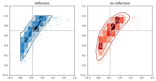
# Load a predefined 2D, 'random' dataset that includes boundaries on both dimensions
data = kale.utils._random_data_2d_03(num=1e3)
# Initialize figure
fig, axes = plt.subplots(figsize=[10, 5], ncols=2)

# Construct a KDE included reflection
kde = kale.KDE(data, reflect=[[0, None], [None, 1]])

# plot using KDE's included reflection parameters
kale.dist2d(kde, ax=axes[0]);

# plot data without reflection
kale.dist2d(data, ax=axes[1], cmap='Reds')

titles = ['reflection', 'no reflection']
for ax, title in zip(axes, titles):
    ax.set(xlim=[-0.5, 2.5], ylim=[-0.2, 1.2], title=title)