Plotting API

For more extended documentation, see the kalepy.plot submodule documentation.

import kalepy as kale
import numpy as np
import matplotlib.pyplot as plt

Top Level Functions

See the below.

kalepy.corner() and the kalepy.Corner class

For the full documentation, see:

• kalepy.plot.corner

• kalepy.plot.Corner

• kalepy.plot.Corner.plot

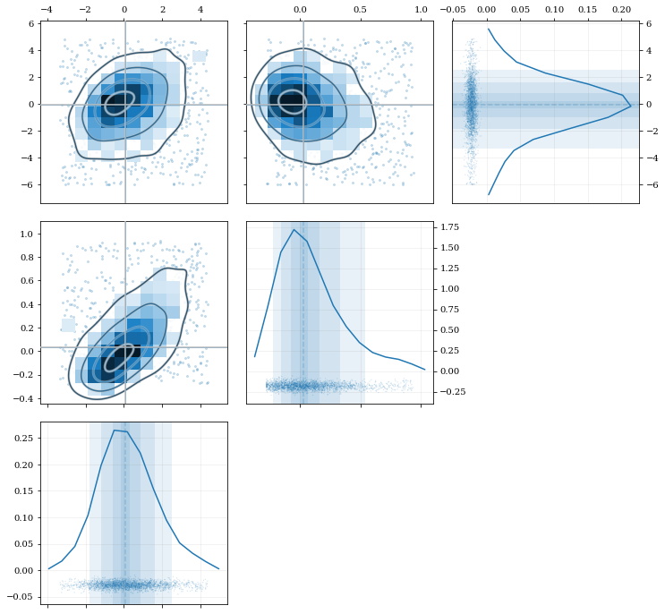
Plot some three-dimensional data called data3 with shape (3, N) with N data points.

kale.corner(data3);

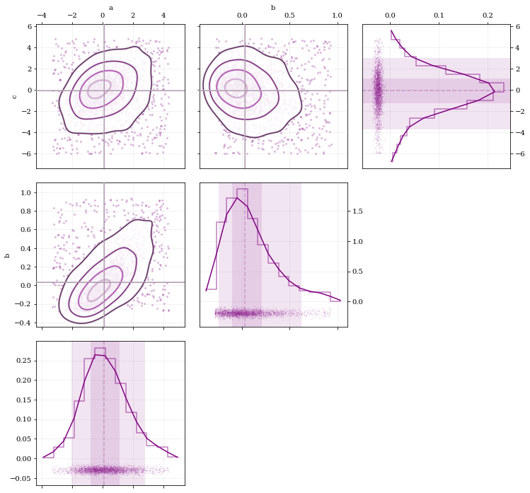
Extensive modifications are possible with passed arguments, for example:

# 1D plot settings: turn on histograms, and modify the confidence-interval quantiles
dist1d = dict(hist=True, quantiles=[0.5, 0.9])
# 2D plot settings: turn off the histograms, and turn on scatter
dist2d = dict(hist=False, scatter=True)

kale.corner(data3, labels=['a', 'b', 'c'], color='purple',
            dist1d=dist1d, dist2d=dist2d);

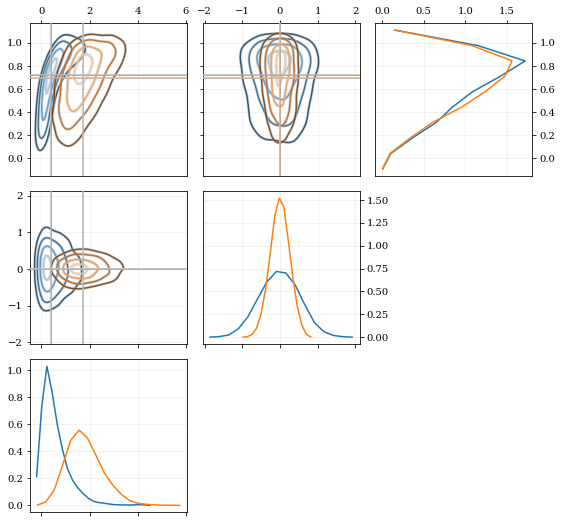
The kalepy.corner method is a wrapper that builds a kalepy.Corner instance, and then plots the given data. For additional flexibility, the kalepy.Corner class can be used directly. This is particularly useful for plotting multiple distributions, or using preconfigured plotting styles.

# Construct a `Corner` instance for 3 dimensional data, modify the figure size
corner = kale.Corner(3, figsize=[9, 9])

# Plot two different datasets using the `clean` plotting style
corner.clean(data3a)
corner.clean(data3b);

kalepy.dist1d and kalepy.dist2d

The Corner class ultimately calls the functions dist1d and dist2d to do the actual plotting of each figure panel. These functions can also be used directly.

For the full documentation, see:

• kalepy.plot.dist1d

• kalepy.plot.dist2d

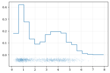
# Plot a 1D dataset, shape: (N,) for `N` data points
kale.dist1d(data1);

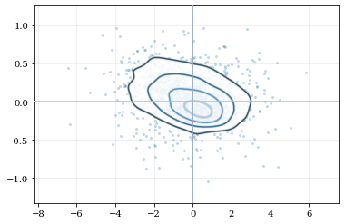
# Plot a 2D dataset, shape: (2, N) for `N` data points
kale.dist2d(data2, hist=False);

These functions can also be called on a kalepy.KDE instance, which is particularly useful for utilizing the advanced KDE functionality like reflection.

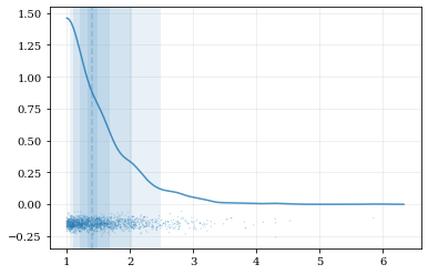
# Construct a random dataset, and truncate it on the left at 1.0
import numpy as np
data = np.random.lognormal(sigma=0.5, size=int(3e3))
data = data[data >= 1.0]

# Construct a KDE, and include reflection (only on the lower/left side)
kde_reflect = kale.KDE(data, reflect=[1.0, None])
# plot, and include confidence intervals
hr = kale.dist1d(kde_reflect, confidence=True);

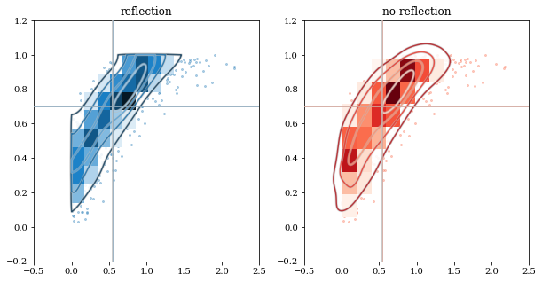
# Load a predefined 2D, 'random' dataset that includes boundaries on both dimensions
data = kale.utils._random_data_2d_03(num=1e3)
# Initialize figure
fig, axes = plt.subplots(figsize=[10, 5], ncols=2)

# Construct a KDE included reflection
kde = kale.KDE(data, reflect=[[0, None], [None, 1]])

# plot using KDE's included reflection parameters
kale.dist2d(kde, ax=axes[0]);

# plot data without reflection
kale.dist2d(data, ax=axes[1], cmap='Reds')

titles = ['reflection', 'no reflection']
for ax, title in zip(axes, titles):
    ax.set(xlim=[-0.5, 2.5], ylim=[-0.2, 1.2], title=title)